Labs

Andrew Anklam                                                                                                                    01/26/2018

Lab 0:

Introduction:

   

     eCognition is a powerful object based image analysis program that can be trained to identify patterns for remote sensing uses. eCognition works by grouping pixels into blocks or objects, the program is then trained by the user to identify classes of objects for the entire image. Once trained eCognition is able to rapidly sort objects in the image. This process of classification allows mapping of say vegetation types to be done cost efficient and rapidly.

Objectives:

• familiarizing our-self with the basics of eCognition by manipulating a Landsat image.          

 Figure 1. eCognition working with satellite imagery

Data Provided: 

• For this lab we are using a Landsat image of Northen Whales. 
• This Landsat image has 6 bands that have a spatial resolution of 25m. 

Methods: 

• Get familiar with eCognition by reading through select parts of the user manual.
• Load satellite image into eCognition and create a project file. 
• Analyze the image by manipulating the bands that are displayed. 
• Experiment with select bands using the equalization function.       

Band Combinations: 

For this section of the lab we were tasked with applying different colors to the 6 different bands from the Landsat and determine what combination would be best for remote sensing purposes.    

Figure 2. Band combination 1. Note how variation within fields stand out.

Figure 3. Band combination 2. Note the visibility of the vegetation around the lakes.

Figure 4. Band combination 3. Note how the fields stand out.

After analyzing each of the band combinations our group decided that band combination 1 was the best for interpreting land use and land cover types because it showed slight variations in land cover types the clearest. The band combination is band 4=red, band 3=green, and band 2=blue.       

Image Equalization:

After determining the band combination that best displayed land cover differences we then applied different equalization to further improve the image analysis. 

Figure 5. Gamma correction equalization.

Figure 6. Histogram equalization.

Figure 7. Standard deviation equalization.

We determined that using the standard deviation equalization was the best equalization for analyzing land cover/land use. The standard deviation allowed us to see the variation in land cover types better than the gamma correction with more variation than the histogram equalization.   

Conclusion: 

After spending some time working with the interface of eCogniton it feels very reminiscent of other image processing based programs like ERDAS or ENVI. Additionally there are some aspects of other GIS programs like the ArcGIS sweet. The one aspect that all of these programs share is the tool bar which is almost identical between ERDAS, ENVI, and eCognition. However eCogniton is most reminiscent of Trimbel programs like GPS office pathfinder which share the same project based saving schema. Like ERDAS and ENVI, eCognition can classify images. However unlike ERDAS and ENVI's image classification which is pixel based eCogntion is object based which can deliver very accurate results when compared to pixel based.   

Figure 8. eCognition's 4 way split function. 

     eCogniton is a powerful program that is like many other GIS programs that I have used. Unlike many other programs that am familiar with eCogniton's functions or tools are treated more like parts that the user assembles to run a analysis. The closest program that I have used that uses functions like this is the ArcGIS model builder. However the model builder is comprised of independent tools as opposed to separate pieces like in eCogniton.

Andrew Anklam                                                                                                                    02/09/2018
Lab 1: Image Segmentation and Nearest Neighbor Classification

Part A

Introduction: 

For this lab I will be working through the full work flow for a nearest neighbor object based image analysis using eCognition. The first part of this lab is focused on the segmentation process in which I preform several segmentation processes using the multiresolution segmentation algorithm with different parameters. The second part of the lab is the rest of the work flow process: classification, sampling, merging, and exporting our final analysis. The final result will be a shapefile that contains the classifications in different polygon classes that can provide us with the area and other spatial deliverable about each classification.         

Figure 1. Results of a experimentation with the multiresolution segmentation algorithm.

Objective: 

• Understand how to produce a nearest neighbor object based classification using eCognition.
• Understand the different parameters in the segmentation and classification process and how they affect the end product.
• Learn how to build complex process trees that automate the object based image analysis process.        

Data Provided:

• For this lab we are using a Landsat image of Northern Whales.
• Unlike in lab 0 we are going to be using the 15 m resolution panchromatic band which has been configured to re sample the Landsat image to bring the resolution of all the bands to 15 m.     

Methods: 

• Load in Landsat image and create a subset of the area around Llyn Brening in Northern Whales. 
• Set up mulit-resolution segmentation algorithm by experimenting with scale, shape, and compactness parameters to produce several different segmentation of the image. 
• Set classification classes: water, forest, other vegetation, not vegetation.
• Set up nearest neighbor classification algorithm to uses selected classes.
• Train nearest neighbor classification by providing samples for each class.  
• Set up merge algorithm to merge all classifications resulting from classification algorithm into the four classes. 
• Set up export algorithm to export classes as a shapefile.
• Run hierarchical segmentation and classification schema.
• Experiment with nearest neighbor classification feature space optimization to fine tune results.
• Produce two maps showcasing the results of the classification process.          

Object Based Image Analysis Segmentation: 

In object based image analysis segmentation is arguably the most crucial part of the work flow. Segmentation is the step where the program groups pixels in the image into groups or objects based on factors like the pixels spectral response or its distance from other similar pixels. All other parts of the work flow process like classification are based off the segmentation results. This is because all pixels that would normally be analysed individually by the classification algorithm are now in these summed up in the objects.                       

Mulit-resolution segmentation experimentation:

This part of the lab focused on understanding how the different parts of the mulit-resolution segmentation process could be manipulated to produce different results. This was achieved by changing the weight or importance of the scale or the acceptable size of the objects, the shape or importance of the objects geometry vs its spectral response, and the compactness of the objects. The fallowing images are examples of the results.
      

Figure 2. Mulit-resolution segmentation high scale (30) results. Note the good segmentation of the forests.   

Figure 3. Mulit-resolution segmentation low scale (8) results. Note how the segmentation appears to be showing the variation withing land cover types. 

Figure 4. Mulit-resolution segmentation high shape weighting (0.9) results. Note the square/block like segmentation.

Figure 5. Mulit-resolution segmentation low shape weighting (0.1) results. Note the segmentation of the groups within the land cover types.

Figure 6. Mulit-resolution segmentation high compactness weighting (0.9) results. Note high segmentation of the fields.

Figure 7. Mulit-resolution segmentation low compactness weighting (0.1) results. Note the segmentation of the forest.

Figure 8. Mulit-resolution segmentation only using the 15 m panchromatic image and setting all weights to 0. 

Based on the experimenting with the parameters for the mulit-resolution segmentation process I determined that the low compactness weight of 0.1 proved to be the best for creating objects based on land cover types. What objects that were created did not overlap land cover types meaning that objects did not contain both field and forest but instead just contained one land cover type per object. However the low compactness weight did create lots of small thin objects on the edges of the lake which is probably the result of the loosely mixed vegetation and water that occurs at the edge of lakes. I assume this problem is only exacerbated the low compactness weight which feeds into the low compact nature of the vegetation on the water.

Figure 9. loose vegetation on the edge of a lake near Växjö Sweden. Photo courtesy of the author.

Part B

NN Feature Space:

In nearest neighbor classification the feature space refers to the statistics in the segmented objects that the nearest neighbor classifies from. For example the nearest neighbor classification could be set to conduct its classification based on the mean spectral response of a object. The maps below are examples of classification using different features.

Figure 10. Nearest neighbor classification using the mean value of each object for its feature space.  

Figure 11. Nearest neighbor classification using the stranded deviation and mean of each object. Notice large areas that were unable to be classified.  

Feature Space Optimization: 

The feature space optimization tool allows for the automatic selection of features within objects that best delineate the classes that have been selected. For this part of the lab I selected different features using feature space optimization and applied them to the classification process.       

Figure 12. Classification after feature space optimization. Features used: mean, stranded deviation, and pixel ratio.

Figure 13. Classification after feature space optimization. Features used: mode, maximum, border contrast.

   

Figure 14. Classification after feature space optimization. Features used: quartile and hue saturation intensity.  

Conclusion: 

Figure 15. Experimenting with segmentation. 

In comparison to lab 1, lab 2 was more about learning how to actually use eCogntion. Lab 1 was about getting somewhat familiar with the layout of eCogntion. Lab 2 detailed how to complete object based image analysis classification workflow enough so I could repeat it on my own. What really helped me understand what exactly I was changing in the algorithms for my classification was the experimenting with the different parameters within each algorithm. This allowed me to connect what theoretically should happen by say setting the shape weight higher to what actually happened in the segmentation process. This learning process could be improved by having the lab focus in on accurately segmenting and classifying one land cover type. This would let people experiment with parameters to figure out what works best. After completing this lab and gaining a understanding of how to conduct a object based image analysis I want to take what I have learned and try to see if its possible to use eCogntion to preform a segmentation on a LiDAR raster data set. This may prove difficult as LiDAR has no spectral data and eCogntion relies on spectral data to an extent for its segmentation process.                    

Andrew Anklam                                                                                                                    02/20/2018

Lab 3: Rule Based Classification

Introduction:

Figure 1. Example of thresholds in class hierarchy

In the last lab we learned how to classify a segmented image by using samples that we provided eCognition. However it is also possible to classify an image using rule sets. These rule sets are structured in two simple types of expressions absolute thresholds and fuzzy thresholds. An example of a absolute threshold are >,<,=,>=,<=, And,or. Fuzzy thresholds are based on degrees from a give value. For example an expression that is meant to classify bogs my look like this: Mean green > 30 meaning that for an object to be considered a bog it must have a mean spectral response higher than 30 in the green band. Using these simple sets of rules its possible to translate knowledge of experts into rules to classify images with. Additionally we will also learn how to create custom features that we can use in our rule based classification like NDVI.            

Objective: 

• Understand what rule based classifications and how to create our own.
• Learn how to create customized features.  

Data Provided:

• For this lab we are using the same Landsat image of Llyn Brening in Northern Whales. Like last time we are also going to be re-sampling the resolution down to 15m using the panchromatic band.

Figure 2. Example of subset.

Methods: 

• Read about rule based classifications. 
• Load in Landsat image and create a subset of the area around Llyn Brening in Northern Whales. 
• Set up NDVI algorithm using the create new arithmetic feature.
• Create new class hierarchy: Acid Semi Improved Grassland, Bog/Heath, Forest, Improved Grassland, Not Vegetation, Water.
• Apply rule sets to each of the classes by inserting thresholds. 
• Set up mulit-resolution segmentation algorithm's scale, shape, and compactness parameters.
• Set up classifications so each class has its own classification algorithm based off its unique rule set.  
• Set up merge algorithm to merge all objects belonging to a class. 
• Set up export algorithm to export results into a shapefile with both class name and area attributes. 

Custom Features: 

Custom features allow the user to enter in their own features which can be used in a variety of functions like classifications. In this case we are going to calculate a normalized difference vegetation index or NDVI. NDVI is a simple equation using the Red and NIR bands (NIR-RED)/(NIR+RED). To do this in eCognition we access the customized features in the feature view window where we are give the option to create our own features. 

    

Figure 3. Setting up custom features in eCogntion. 

Rule Set Classification:

the real strength of the rule set classification comes from its easy manipulation and simple encoding of rules. Additionally it removes the process of creating sample points which can be a time consuming process. Each of the class were assigned different rules like the fallowing rule set for improved grassland class: Mean NIR > 100.

Figure 4. Results of the rule set classification. 

Segmentation Experimentation: 

By experimenting with the segmentation parameters its possible to change how the rule based classification will turn out. Below example are some examples of how changing the parameters can change the end classification.    

Figure 5. Rule set classification after changing segmentation parameters. Scale: 30 Shape: 0.9 Compactness: 1 

Figure 6. Rule set classification after changing segmentation parameters. Scale: 1 Shape: 0.3 Compactness: 0.7 

Figure 7. Rule set classification after changing segmentation parameters. Scale: 15 Shape: 0.5 Compactness: 1   

Classification improvement:

Despite the relative ease of classification our rule set classification has several errors within it. In an attempt to improve the accuracy of the classification several thresholds were modified with varying results.     

Figure 8. Experimenting with rule sets to improve classification. Note how there is less of the "Not Vegetation" class in the water.  

Figure 9. Experimenting with rule sets to improve classification. Note how there is large chunks of unclassified objects, this resulted from setting a greater then threshold on the "Acid Semi improved Grassland" class.

Figure 10. Experimenting with rule sets to improve classification. Note how the "Not Vegetation" class has been removed. This resulted from adding a must be less than threshold to the NDVI feature in the rule set.

After trying several modification of the rule set classification the classification was only slightly improved from the experimentation. For example the modifications in figure 8 only removed a few sets of miss-classified objects around the lake but also caused a few grassland classes to become the semi improved grassland class. The other two modifications in figures 9 and 10 both suffered as some of the classes simply disappeared or fail to classify.   

Improvement: 

After some more modification with parameters outside of rule based classification and some more analysis of the failed modifications the rule set classification was improved.

Figure 11. Improved rule set classification. 

   The first aspect of the classification that was changed was the segmentation scale parameters which were changed from 10 to 15 then to 12. This change allowed for the removal of  tiny objects that would form around the edges of the lakes and sometimes forest which tended to be classified as not vegetation. After setting the segmentation parameters several classification errors were analysed by looking at the mean spectral response for each band. This lead to the modification of the "Forest" SWIR 1 threshold to be less than 48 (SWIR 1 <48) and the "Not Vegetation" SWIR 2 to be greater than 40 (SWIR 2 >40). These changes caused the classification of the "Forest" and "Not Vegetation" classes to improve as they no longer had a few miss-classified objects in them.

Figure 12. Original rule set classification.

     Conclusion: 

Rule set classification is a easier to understand classification than the nearest neighbor classification that we did for lab 2. Understanding the basic principles of remote sensing and structured query language coming into this lab made learning and modifying rule sets easy. However the rule set classification is less flexible than the nearest neighbor classification that was conducted in lab 2. It was possible to refine the results further in the nearest neighbor classification than in the rule set classification. After trying to improve the rule set for hours it felt like the classification was static and becoming more confusing as entering new rule sets failed to produce the predicted results. 

      Another strength of rule set classification is its ability to encode knowledge (rules) into the classification. This lab although it demonstrated how this was possible failed to include any application of this. In the future it would be helpful for this lab to include a section were properties about a land cover type is given and the participant has to encode these properties into a rule set.         

Andrew Anklam                                                                                                                    03/04/2018

Lab 4: Converting DN to Reflectance and Atmospheric Correction of Landsat 5 TM

Introduction: 

spectral data from every space based remote sensing platform has to deal with errors in their data caused from distortion of the spectral response by particles. These errors are caused from aerosols, water vapor, or other particulates that cause scattering of light. light can be distorted in a verity of ways like additive scattering or multiplicative transmission. To adjust for the error caused by the atmosphere most satellite data is preprocessed before it is distributed to remove the error and display the DN as if it was recorded near the surface. However some older satellites did not preprocess the data leaving it up to the user to correct for the atmospheric distortion.

     For this lab we will be taking uncorrected Landsat 5 TM data of La Crosse Wisconsin and apply a DOS and COST atmospheric correction model to produce two sets of NDVIs.              

Figure 1. Landsat 5 TM scene in ERDAS. 

Objectives: 

• Become familiar with the concepts of atmospheric scattering and correction of atmospheric scattering.
• Understand how to use ERDAS modeler for the correction of satellite images.
• Learn how to calculate radiance, top of atmospheric reflectance, and surface reflectance from a uncorrected Landsat image.       

Data Provided:

• We are provided with a 30m resolution Landsat 5 TM image of the greater La Crosse area which has a total of 6 bands. This image has not been corrected to account for the effect of atmospheric scattering. 
• Additionally a COST model has been provided to correct for atmospheric scattering. The COST model is in excel format.  

Methods: 

• Load Landsat 5 TM scene. 
• Analyze the metadata for the date of acquisition, sensor ID, cloud cover, sun azimuth, sun elevation angle, radiance values, solar zenith angle, and quantize cal values.
• Using ERDAS' modeler function create a model to convert the raw Landsat 5 TM image DN to radiance.
• Modify the modeler to convert radiance into top of atmospheric (TOA) reflectance.
• Enter values from metadata and TOA reflectance into the COST excel correction model. 
• Create the COST correction model in ERDAS' modeler to produce surface reflectance.
• Create NDVIs using the output layers in modeler. 

Figure 2. Landsat 5 TM metadata being viewed in WordPad.

    Metadata: 

Metadata or data about the data is key to understanding any kind of remote sensing data. In this case the Metadata for the Landsat 5 TM is delivered as a separate text file with the image. For this part of the lab we opened the data in WordPad to get the fallowing data. , radiance values, , and quantize cal values.

• Date of acquisition: 04/10/1993    
• Sensor ID: TM
• Cloud cover: 0% 
• Sun azimuth: 148.16 degrees 
• Sun elevation angle: 35.844 degrees
• solar zenith angle: 54.156 degrees

Additionally the radiance values and quantize cal values were recorded and used later for calculations.

ERDAS modeler: 

ERDAS' modeler function similar to the modeler function in ArcMap is a visualized workflow tool set that allows the user to build and automate complex functions. For this lab we are going to be using ERDAS to modeler to build and execute band math on the Landsat 5 TM image to produce a corrected image. 

      

Figure 3. Example of ERDAS' model builder.

The first function that needs to be preformed in ERDAS is building the equation to convert the DNs in the uncorrected image to radiance or the amount of energy radiating off the surface imaged. To do this the a function is applied to each band and then stacked into a new band. 

• DN to radiance formula: (((193.0)-(-1.52))/(255-1))*($n1_lt50260291993277xxx02_subset(1)-1)+(-1.52)  

      

Figure 4. DN to radiance formula in ERDAS modeler.

After creating a image with radiance for each band we need to import the new radiance image back into ERADS modeler to convert the image from radiance into top of atmospheric reflectince. The model is similar to the radiance model but there is an extra set of conditional functions to remove any negative values. 

• Radiance to TOA reflectince: ($n1_radiaince_model(1) * PI * 1.00119 ** 2) / (1957 * COS (PI/180 * (90 - 35.84416315))) 

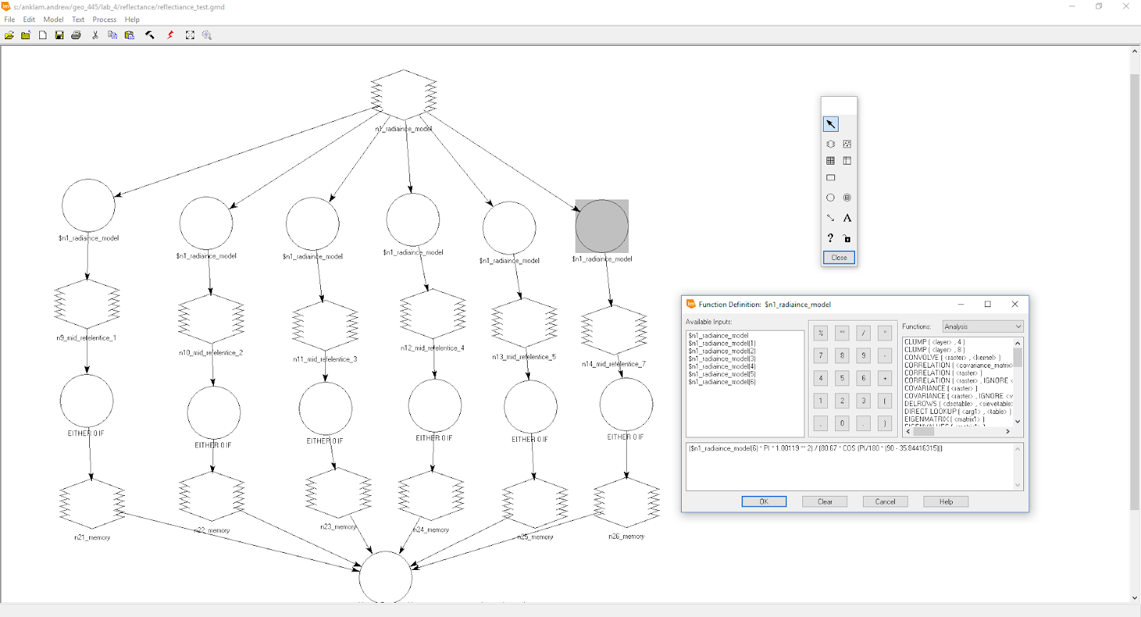Figure 5. Radiance to TOA reflectince ERDAS model. 

The final step to produce the corrected surface reflection is to enter the values calculated in the TOA reflectince image and values contained in the metadata into the COST excel model. The COST model provided is a improved version of atmospheric correction that accounts for multiplicative transmission scattering as well as additive scattering unlike DOS and DOS improved corrections models. See Chavez 1996 for more details on how this correction is done.     

• TOA to surface reflectince: (($n1_radiaince_model(1)-(22.3182730))*PI*1.00119**2)/(1957*COS(PI/180*(90-35.84416315))*0.7) 

Figure 6. COST correction model in excel.

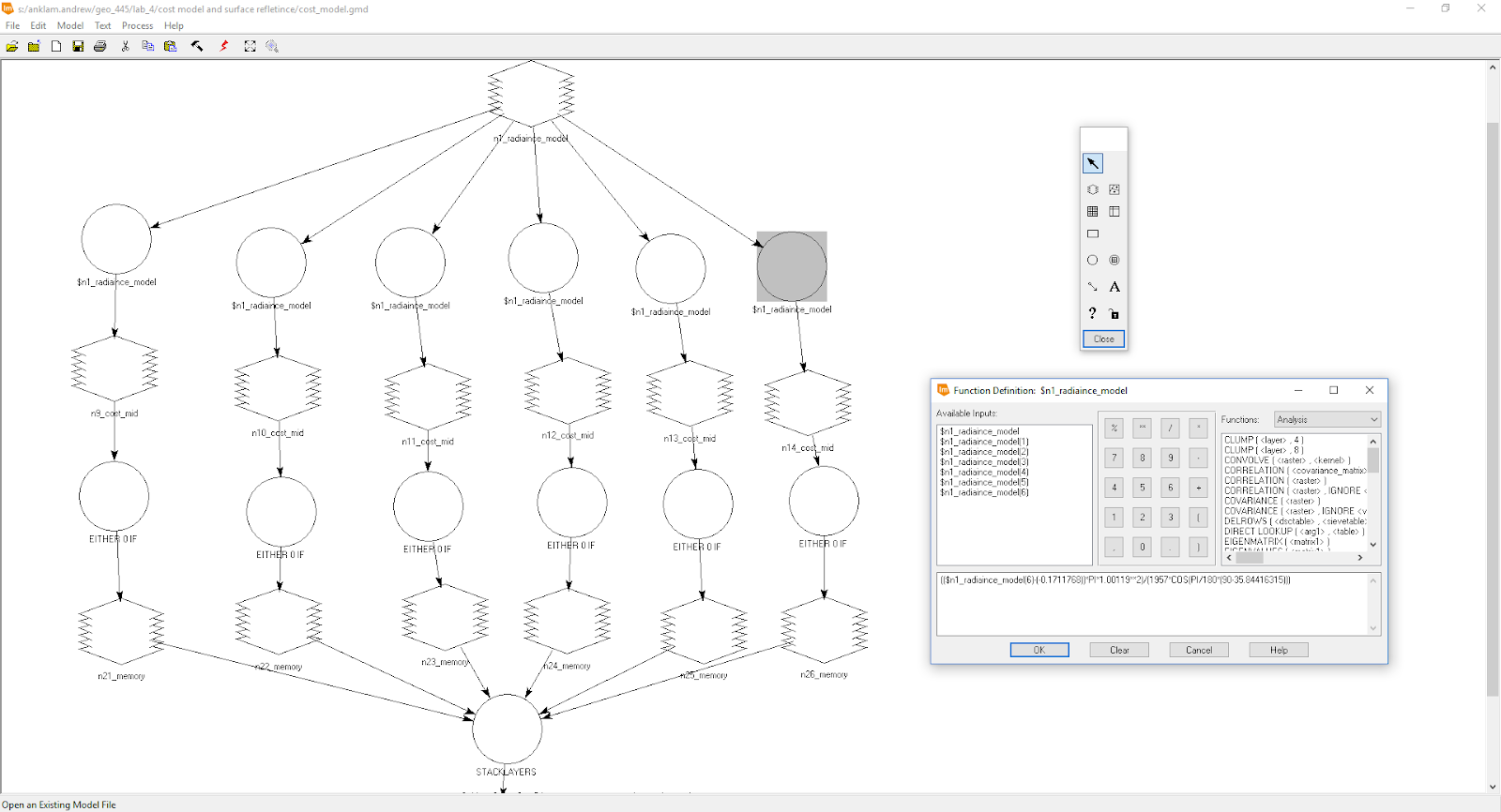Figure 7. TOA reflectince to COST surface reflectince in ERDAS modeler.

NDVIs:

After calculating the corrections for the Landsat 5 TM image 3 NDVIs were made using the radiance image, the TOA reflectince image, and the COST surface reflectince image in ERDAS modeler. Additionally tables showing various pixel values with in each NDVI were created. 

Figure 8. NDVI calculation in ERDAS modeler.

  

Figure 9. Example of a NDVI in ERDAS.

Table 1. Table showing values of bands in the COST surface reflectince.

Band #	Minimum reflectance	Mean reflectance	Maximum reflectance	Standard
1	0.0056	0.047	0.498	0.016
2	0.0020	0.047	0.461	0.019
3	0.0000	0.012	0.363	0.012
4	0.0007	0.131	0.355	0.046
5	0.0003	0.020	0.069	0.007
7	0.0005	0.004	0.027	0.002

Table 2. Table showing values of various pixels in the NDVIs.

Pixel	Row #	Column #	NDVI from raw DN	NDVI from reflectance
1	423.8257	512.6565	0.289	0.622
2	485.6900	769.6313	0.672	0.768
3	836.2544	1418.4134	-0.357	-0.169
4	35.8733	1791.4922	0.223	0.405
5	831.4782	1628.8483	0.237	0.417
6	994.8283	72.8691	0.444	0.591
7	247.2938	153.1599	0.308	0.0478
8	322.0473	925.6121	0.227	0.409
9	850.8587	1941.7053	0.444	0.592
10	950.5300	1343.6777	0.390	0.547

While analyzing the NDVIs a few patterns became apparent. First the reflectance values of the raw DN NDVI were always less than than the values from the TOA reflectance values. Additionally the difference between the pixel values tended to differ the most on crop land while they were the most similar on water. This appears to be because water is a relativity homogeneous land cover type while crop land is a heterogeneous land cover type allowing for more variation in pixel value.

Figure 10. Rapeseed crop land near Kalmar Sweden, Notice how spacing between plants allows for a heterogenous land cover type. 

Conclusion: 

Coming into this lab I had some prior experience using ERDAS and some bref albeit simple understanding of ERDAS modeler. However I should note that I did have a fair amout of experience using similar modeling programs like ArcMap to automate workflows. While working with ERDAS I had to relearn most functions but was able to quickly remember them.

     Working with ERDAS in combination with the Landsat 5 TM metadata at first seemed very conceptual and hard to visualize. However by the time we started the second conversion function the concepts we were working with and the equations we were building started to become understandable in their context. Understanding the concepts in the lab would of not been possible without building these functions in ERDAS' modeler. However the actual building of the functions in modeler proved to be extremely frustrating as simple syntax errors like adding a extra bracket would cause the function to fail. This was made worse by the vage error messages which did not really tell what the specific error was. In future iterations of this lab I would suggest adding a section in class where everyone builds the function at the same time while a example is also being built on a projector in front of the class. After working with these functions in ERDAS to correct satellite image error I now have a solid understanding of the concepts and functions behind correcting atmospheric scattering.                               

Andrew Anklam                                                                                                                    03/23/2018

Lab 5: Spectral Mixture Analysis

Introduction: 

     The mixed pixel problem has hindered almost all remote sensing applications as the basis for almost all remote sensing applications is the pixel. The mixed pixel problem states that within each pixel is a variety of land cover types but the land cover type that takes up the most of the pixel is the one represent in the values of the pixel. This can result in a pixel that is split 40-60 only displaying the values for the land cover type that takes up 60% of the pixel. 

     Spectral mixture analysis is one way to circumvent the mixed pixel problem. Spectral mixture analysis (SMA) functions under the assumption that every image has a pure or endmember pixel of a land cover type. These endmember pixels can be identified to give an idea of what the spectral response for each land cover type is like in each image. By identifying the spectral response for each land cover type from the endmember pixel, other pixels in the image can be broken down by band and assigned a percent of land cover type based on the spectral response of each band in the pixel. The process of SMA can provide better classification of images than regular mixed pixel analysis as pixels can be broken down to show percentages of land cover types within each pixel.
     Lab 5 involves us learning the basics of selecting endmembers, unmixing pixels, and assessing the accuracy of the unmixing using ENVI classic.            

Figure 1. ENVI classic being used to visualize a Landsat image of the La Crosse area.  

Objectives: 

• Learn the basics of spectral mixture analysis.
• Learn the different types of spectral mixture analysis.
• Learn how to select endmember pixels and develop a spectral libary.
• Understand how to apply the spectral libraries to conduct a spectral mixing analysis. 
• Understand how to determine the accuracy of spectral mixture analysis.

Data Provided:

• We will be conducting our SMA on a subset of a Landsat 8 image of La Crosse Wisconsin which has a resolution of  30 m and contains 5 spectral bands.   
• The Landsat 8 subset has already been corrected to show top of atmosphere (TOA) reflectance values. 

Methods:

• Load in and explore the Landsat 8 subset into ENVI, checking the metadata and image. 
• Set the Landsat 8 subset to a true color composite.
• Consider the accuracy of unmixing pixels with certain types of land cover.
• Select some endmembers using a scatter plot of pixel reflectance and export them to a spectral library.    
• Select some endmembers by selecting regions of importance (ROI) and exporting them to a spectral library.
• Combine spectral libraries and unmix image using the combined spectral library.
• Analysis unmixed image to determine accuracy of the SMA.       

Unmixing Pixels and Perceived Accuracy (Question 1): 

Before we start gathering spectral libraries and unmixing the image it is important to consider how well certain types of land cover will be represented in each pixel. For example a pixel that contain both water and vegetation like cattails might have a low unmixing accuracy because of how heterogeneous the two land cover types are. Another example is when two land cover types have a similar spectral response in a band which could cause the unmixing to wrongly classify some of the more heterogeneous pixels.      

Figure 2. Spectral plot showing the spectral response of green vegetation and bare soil. 

Table 1. Table showing the hypothesized separability between land cover types 

for SMA.

	Water	Green Vegetation	Bare Soil	Built  Up
Water	None	Low	High	Medium
Green Vegetation	Low	None	Medium	High
Bare Soil	High	Medium	None	Medium
Built Up	Medium	High	Medium	None

Selecting Endmembers With Pixel Scatter Plots:

Endmembers or a "pure" pixel is a pixel comprised of only one land cover type. In SMA endmembers are how we can determine how each land cover type reflects in each band. By knowing how say water reflects in the blue band it would be possible for us to pull the percent of water in a pixel out by the way the pixel is reflecting in the blue band. However truly "pure" endmembers are hard to find in the real world, becoming increasingly hard to find with larger pixel sizes.

     One way to find endmembers in a image is to make a scatter plot of all the pixels in a image. For this lab we were able to identify the endmembers for green vegetation by creating a scatter plot of the spectral response of the red and near infrared bands. Because we know that green vegetation reflects highly in the near infrared band and not that much in the red band we can be confident that pixels with this spectral response are comprised almost entirely of green vegetation. 

Figure 3. Scatter plot of the near infrared band (y axis) and red band (x axis) pixel's spectral response of the La Crosse subset. Note the circled area on the top is the selection of endmembers for green vegetation.

    

     After selecting the green vegetation endmembers in ENVI we can now save them as a spectral library. Later we will add this spectral libraries to create a completed spectral libraries.

Selecting Endmembers With Regions of Influence:

Region of influence or ROIs are user defined region (polygons) that act like samples for whatever analysis is going to be conducted. In this case our ROIs are going to be used as endmembers. However before we select a ROI it is important that to make sure that what we are selecting pixels that are comprised of the land cover we think they are. One way to determine that pixels are homogeneous is to enhance the image with different filters. 

Figure 4. A Gaussian enhancement applied to the La Crosse subset. Notice how water that appears to be homogeneous in a true color composite can actually be "clouded" and is visible in various enhancements.   

Once we have found an area with homogeneous looking pixels we can define our ROI.

Figure 5. Defining an ROI in ENVI. 

     Using this process of defining ROIs, endmembers for water, bare soil, and built up land cover types were defined and saved into spectral libraries.

Unmixing The Image: 

     After we have defined all of our endmembers for each of the land cover types we need to compile the resulting spectral libraries into one spectral library that we can apply to our image to unmix it. Using ENVI's spectral library builder tool we can combine all the spectral libraries into one spectral library.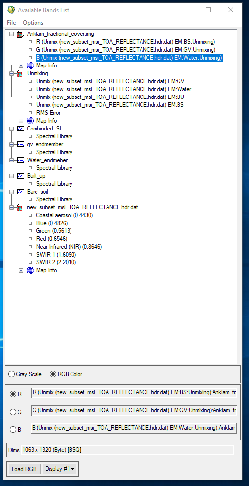

Figure 6. Spectral libraries displayed in ENVI's table of content.   

         

Figure 7. Resulting spectral signatures from the final spectral library. 

Using this complete spectral library we can now import it into ENVI's liner spectral unmixing function to unmix the image. 

Figure 8. False color composite of the unmixed image.

Accuracy Assessment: 

    Once we have conducted the unmixing of the image we need to check to see if our unmixing models that we created with the selection of endmembers is accurate. One way to do this is by analyzing the pixel data values for random pixels. Ideally the data values should be near to zero. Data values can be though of as the distance of the pixel value from the predicted value derived from the model. This means that a observed value close to zero in our unmixing is close to the predicted value. 

Figure 9. Example of data values from the unmixed image. Note that the blue band has the most inaccuracy, the green band has a negative value, and the red band is the most accurate.  

Additionally it is possible to access the accuracy of the unmixing by loading in the RMS Error band produced by the unmixing process in a gray scale. By analyzing the data values form this layer it is possible to derive the the random mean square error of each pixel. The further the value is form zero the less accurate the unmixing is for the pixel.

Figure 10. RMS error visualized in ENVI as a grey scale to check unmixing accuracy. 

        

Question 2: 

Q: Are your fractional cover values in negative? Why do you think they are negative?             

A: Some of my fractional cover values are negative. This is because the unmixing model is over predicting for the data values of some of the pixels. Imagine a scatter plot of all the data values and a linear trend line running through the scatter plot. The linear line is the model's predicted values and the points are the observed values. values under the line will appear negative and values above the line are positive.

Question 3: 

Q: Which fractional cover type do you think has lowest accuracy? How will you access the accuracy of fractional cover estimates? 

A: The lowest land cover accuracy came from both the built up and bare soil land cover classes. The accuracy was accessed by analysis of the RMS error band's pixels values. The closer the data value was to zero the lower the RMS error was. This means that the closer the data vale was to zero the better our model is at predicting the unmxing values.    

Conclusion: 

Before doing this activity I had very little knowledge of both spectral unmixing and ENVI, although I knew that ENVI was similar to ERDAS. However after completing this lab I feel familiar with ENVI enough that I understand and am now comfortable using it. I also know have a solid understanding of the concept of spectral mixture analysis as well as how to understand if the unmixing is accurate. 

     By working through this exercise in class and on my own I was really able to develop a understanding of how the theoretical ideas behind spectral unmixing are applied. Before doing the lab I probably could of figured out how to do a spectral mixture analysis but would of had no idea of what I was doing. One thing that really helped my understanding of how the spectral unmixing was being done was assessing the unmixing. By working with the errors it helped me make the connections about the different concepts in spectral mixture analysis. To further improve this lab I would suggest using an image with more spectral bands, whether it be super spectral or hyper spectral. This would give students a better understanding of what the potential is for spectral unmixing.     

    After working with ENVI and SMA its easy to see to applications for SMA. Besides the general applications to improve the classification accuracy SMA could be applied to fine tune classification, delineating between vegetation or mineral types based on slight changes in various bands. As an archaeologist I can see the use of SMA to pinpoint soil stains on bare soil to delineate archaeological features. It will be interesting to see where SMA and spectral unmixing goes in the next few years.   

Andrew Anklam                                                                                                                   04/03/2018

Lab 6: MODIS images and data processing in ENVI

Introduction: 

     The MODIS sensor series is a valuable tool for remote sensing scientists trying to understand large scale changes occurring on earth. MODIS is a spectral sensor mounted on a set of two satellites, Terra and Aqua which are apart of the earth observing system. Unlike other satellites Terra and Aqua image every part of the earth about once a day meaning that the MODIS sensor has a unparalleled view of the day to day changes that occur on the surface of the earth. The MODIS sensor has proven to be invaluable for understanding vegetation patterns partly because of its day to day imagining and that it images in 32 spectral bands ranging in resolution from 250 m to 1000 m. The wide array of spectral bands allows MODIS to be applied to study anything from weather patterns to vegetation growth. 

     Because of shear amount of uses that raw MODIS imagery can be applied to it is important to understand how to pre-process the data for its specific use. Thankfully its possible to get data from NASA serves partially pre-processed however this data still needs to manipulated in programs like ENVI before they can be used in programs like TerrSet to conduct analysis. For this lab we are going to be learning about and processing MODIS data in ENVI so it can be used in lab 7.             

Objectives:

• Learn how to work with MODIS data.
• Understand concepts influencing MODIS data. 
• Create a layer stack of 17 years of growing data from MODIS.
• Pre-process data for use in lab 7.

Data Provided:

• The data used in this lab is a image of the upper midwest form the MOD13C1: MODIS/Terra Vegetation Indices series.
• The data has been pre-processed by the distributor into a 500 m resolution yearly compost of the growing season.      

Figure 1. Visualization of this lab's MODIS image.

Methods: 

• Collect 17 MODIS growing season composite images from NASA's MODIS data portal Earthdata. 
• Stack the 17 MODIS growing season composite images using ENVI's layer stacking function.
• Scale the stacked image by a scale factor of 1000 using ENVI's spectral math function.
• Mask the image using ENVI's masking function to replace all negative values with 0.
• Convert the resulting file into a 16 bit unsigned integer using ENVI's band math function.
• Re-scale the image back down by a factor of 0.0001 for export to TerrSet.  
• Analysis the data to determine the quality of the pre-processing.       

Gathering data: 

The first step in this lab is getting a hold of the data. MODIS data is made freely available through NASA's Earthdata data portal. Once on Earthdata the area of interest can be selected using a interactive web map that allows the user to define the area and what type of data to request. 

Figure 2. Selecting MODIS data using the Earthdata data portal.

     Once the data is selected to our parameters it is sent to a NASA processing server where it is processed then delivered to the user via email. 

Stacking the image: 

Now that we have the data from Earthdata we need to stack all 17 images into one layered image. To do this we use ENVI's layer stacking function. 

Figure 3. Stacking images into one layer image in ENVI.

 After the images have been stacked they can be brought into ENVI and worked with as one image with multiple bands.

Spectral math: 

MODIS images come scaled down by a scale of 0.0001 to save space when processing and moving the image. To make the image easier to work with we need to rescale the image back up by a factor of 1000. To do this we will use ENVI's spectral math function which applies mathematical functions to each specified band through an entire image as opposed to by individual layer bands as is done in band math. 

Figure 4. Applying a scale factor of 1000 to the image using the spectral math function.

         Now that the image is scaled up the image is easier to work with. 

Masking the image:

For our analysis in lab 7 we only want to work with pixels that have a positive NDVI values through out the 17 years. In order to cut out all pixels with negative values we need to build a mask that will apply an expression to our image that will reassign the value of all negative values to zero and all positive values to 1. To do this we need to use ENVI's mask builder to enter the mask then apply the mask to the image.

Figure 5. Building the making layer using the mask building function.  

Once the mask is made it must then be applied to the stacked image.

Figure 6. Applying the mask through selecting the image and mask.

Figure 7. Applying the masking values to the selected image.

    

Figure 8. Masked image. Notice how the value of water pixels that used to be negative now appear as 0.

Re-scaling and unsigned integer:

The final step in our pre-processing is to rescale the image back down by a factor 0.0001 and convert it into a unsigned integer. For use in TerrSet we want our data in a 16 bit unsigned integer meaning that the data cannot be negative and range in value from 0 to 65,535. To scale and convert our data we again need to apply a expression using spectral math. 

Figure 9. Applying the conversion expression to the masked image.  

    Data analysis: 

Question 1: What are two limitations of NDVI band ratio. 

Answer: NDVI band ratios are really only good at looking at a moderate amount of vegetation. NDVIs can produce over saturated results when there is a large amount of vegetation preset in the image skewing the resulting ratio. Additionally the opposite of this can also happen when there is too much soil visible in the image resulting in a poor NDVI ratio.

Question 2: 

Create a spectral plot of this location 43.80626 N, -91.201492E for the years 200, 2005, and 2015 using the stacked 10000 scaled image.     

Answer: 

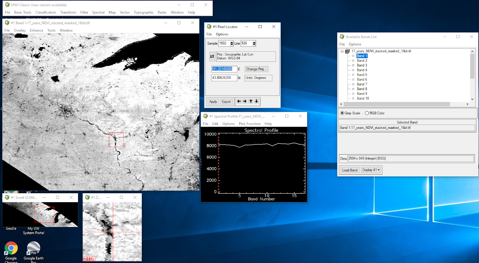Figure 10. Spectral profile the mean scaled growing season year 2000. 

Figure 11. Spectral profile the mean scaled growing season year 2005. 

Figure 12. Spectral profile the mean scaled growing season year 2015. 

Question 3: 

Create a spectral plot of this location 43.80626 N, -91.201492E for the years 200, 2005, and 2015 using the stacked re-scaled image.   

Answer:

Figure 13. Spectral profile the mean re-scaled growing season year 2000.

Figure 13. Spectral profile the mean re-scaled growing season year 2005.

Figure 14. Spectral profile the mean re-scaled growing season year 2015.

Conclusion: 

After the last lab I had a much greater understanding of ENVI and would consider that I had a good understanding of ENVI but had little understanding of MODIS data. However after completing this lab I now have a moderate understanding of working with MODIS data and a very good understanding of ENVI. While working though this lab with the instructor I was able to efficiently work though the lab. However while doing the write up I found that I had to go back several times to revisit some steps as we went through these sections very fast during the in class section of the lab. In order to improve this lab I would give the students a bit more self guided time with the lab. Still include the demos at the beginning of the lab but let students finish the last half.
     ENVI is a useful tool for working with raster data. It is a powerful processor of data but is relatively simple to operate. In this case ENVI was use to effectively pre-process the data for its import into TerrSet.              

Andrew Anklam                                                                                                                  04/013/2018

Lab 7: TerrSet Analysis Using MODIS data

Introduction: 

 In Lab 6 a series of MODIS image were processed to work with in TerrSet. Lab 7 involves taking the data produced in lab 6 and running an analysis on it in TerrSet. TerrSet is a powerful geo-modelling program that can be used to model climate change or long term land change. Unlike some of the modeling functions built into ArcMap or ENVI, TerrSet has several complex and specific modeling functions built into it requiring less processing to make a end product. However TerrSet has very little visualization function meaning that Processed TerrSet data needs to be post processed in programs like ArcMap or ENVI.   

      For this lab we will be using TerrSet's earth trend molder to model the significance and intensity of greening and browning in Minnesota and Wisconsin. To do this the MODIS data needs to have a liner trend OSL run on it to determine the 'slope'/intensity of the browning and greening as well as a Mann-Kendall significance test to determine the significance of the browning and greening . Once the data has been processed in TerrSet it must be exported to ENVI and ArcMap to be post processed.       

Figure 1. Loading files into TerrSet.

Objectives: 

• Understand the concepts of OSL and significance.
• Apply OSL and significance to MODIS and geospatial data.
• Learn how to use TerrSet. 
• Produce and interpret a vegetation trend map of Minnesota and Wisconsin.  

Data Provided:

• The final image made in lab 6 will be used as the input for lab 7.
• This image was a 16 bit unsigned integer containing a MODIS composite mean growing season NDVI for the upper Midwest.     

Figure 2. Final image from lab 6.

Methods: 

• Create a project in TerrSet and import the final image from lab 6. 
• Convert the imported image into a time series file .TSF.
• Preform a series trend analysis with a liner trend OSL analysis and a Mann-Kendall significance test.
• Export the resulting file to ENVI to apply the significance to the OSL trend. 
• Use ArcMap to reclassify and create a trend analysis map. 
• Interpret the results of the trend analysis map.       

TerrSet:

Once we have converted the image into a tif file we can import it into TerrSet's earth trends modeler (ETM). Using TerrSet's browser a project filed is created where the image is stored. The image is then converted into a time series file which treats each band of the image as a year that is then used in the model. 

Figure 3. Visualization of a time series file in TerrSet's ETM.

Now that the model is in a time series file it can now be analyzed with ETM. In ETM the time series file file is analyzed using a liner trend OSL and Mann-Kendall analysis. Liner trend OSL can be though of as a trend analysis that determines the overall trend of the data or this case the trend of the browning and greening. Mann-Kendall analysis can be though of as determining the significance of  the observed trend.

Figure 4. Running a liner trend OSL in TerrSet's ETM.

Post-processing in ENVI:

After running the OSL and Mann-Kendall analysis in TerrSet the resulting files are exported as a tif file to be post-processed in ENVI. Once in ENVI the OSL file which represents slope of the observed trends need to be applied to the Mann-Kendall significance values. To do this a band math expression is applied to the two images.      

Figure 5. Applying significance to the observed trends using a band math expression.   

This band math expression states that if band 1 (the Mann-Kendall test) has a alpha value of less than 0.05 then the OSL trend is significant and is not the result of a normal seasonal browning and greening trend. In other words its like saying that we are 95% confident the these greening and browning trends are not the result of seasonality.     

Figure 6. Applied band math function visualized in ENVI. 

Post-processing in ArcMap:

Once the data has had the band math expression applied in ENVI it must be interpreted in ArcMap. Using the reclassify tool the values in the image can be put into meaningful classes. For this classification the following parameters will be used. 

Table 1. Reclassification values.  

Original data values	New data values	Meaning
-300 – -75	1	Intense browning
-75 – -0.01	2	Mild browning
-0.01 – 0.01	No data	Little to no change
0.01 – 75	3	Mild greening
75 – 300	4	Intense greening

    

Figure 7. Reclassifying image in ArcMap. 

After reclassifying the image a map was made to show the trend of greening and browning in Minnesota and Wisconsin.

Figure 8. Greening and browning trends in Wisconsin and Minnesota from the years 2000 to 2017.

  Now that the file has been clipped and interpreted its possible to quantify the greening and browning trend in Wisconsin and Minnesota.

Question 1: 

How much area within Minnesota and Wisconsin showed statistically significant negative (browning) trend?

Answer: There was a total of 16,331 square km of browning in both Wisconsin and Minnesota between the years 2000 and 2017.

Question 2: 

How much area within Minnesota and Wisconsin showed statistically significant positive (greening) trend?

Answer: there was a total of 20,530 square km of greening in both Wisconsin and Minnesota between the years 2000 and 2017.

Question 3: 

What was the highest magnitude and lowest magnitude for observed greening and browning pixel?

Answer: The highest magnitude browning observed was -426 and the lowest magnitude browning observed was -0.58. The highest magnitude greening observed was 366 and the lowest magnitude greening observed was 2.5.   

Question 3:

Preform a spatial analysis and report how much area of these categories were present in each land use land cover category. 

To complete this question the reclassified map needs to be brought back into ENVI and compared with a land cover land use image. By taking the reclassified image and applying a coded land cover image subsets were defined by each land cover code. These subsets could then be used to analyze the trends in each land cover class. 

Figure 9. Applying a land cover image to the browning and greening trends. 

Answer: 

Table 2. Area in square km of browning and greening trends by land cover class

Land cover name	Intense browning	Mild browning	Mild greening	Intense greening	Total area with significant trend
Mosaic cropland	146	597	13	280	1036
Rainfed cropland	110	11	141	50	312
Mosaic grassland	128	16	175	33	352
Mosaic forest	134	12	339	80	565
Mosaic vegetation	2484	200	1855	451	4990
Evergreens	162	24	96	6	288
Deciduous forest	13993	2325	17941	2548	36807

    

Conclusion:

Before starting this lab I had very little knowledge of TerrSet and its functions, however after working with it for some time I am now somewhat confident with useing TerrSet on my own. It was interesting to see how TerrSet applied other ideas that we had learned in other classes like significance tests and calculating slope to raster data. It feels like TerrSet is a very robust tool diffrent from other tools that have been integrated into ArcMap. While working on the lab I found it crucial that the instructor explained exactly what we were doing in TerrSet. without this knowledge I would have had a hard time understanding what exactly I was doing in TerrSet. However I would of found it helpful if the instructor reviewed the data that we made in the last lab before starting this one. Aspects of the last lab were slightly unclear like whether or not we were going to be working with the scaled image or not. I found this introduced some uncertainty into the this lab.

    After completing this lab I am able to understand how to apply different functions like statistical significance of raster data. In the future I would like to take the methods I learned in this lab to determine the significance of my own data sets.